Working With Data
Dai Shizuka
updated 09/02/25
Overview
Most of you are looking to use R for data analysis, which of course requires learning how to import your data into R. This is maybe the big leap for people who are not used to programming.
To import data into R, you will create an object that points to a dataset somewhere on your computer. R will then import that data as a dataframe object (see Module 2).
1. Importing Data: Overview
Do this before you start this section (if you didn’t do it in the previous module)!
- Click on this link to download a zip file:
- Unzip the file. YOu will find a folder called “data”. Put this inside your working directory (i.e., the folder where you are keeping all of your course materials)
1.1 File Formats for spreadsheets: Using .csv (or .txt)
Many of us manage data by entering them into a spreadsheet using common software like Microsoft Excel. While we have all likely had headaches associated with Excel, it’s undeniable that it is still the predominant way to compile our data.
R can read several file formats, but the popular excel format (.xls
or .xlsx) is NOT one of them (unless you use a specialized package,
e.g., xlsx). Instead, you will most often convert your
excel sheet into one of two formats: tab-delimited files
(saved as .txt) or comma-separated-values
files (.csv). These are simple text files in which each
entry is separated by a tab or comma (respectively). The huge advantage
of these formats is that they are non-proprietary file
formats that can be read by any text editor. This is super
important: .xls or .xlsx file is only useful
on computers with Microsoft Office software, .csv or
.txt file is universal, and anyone with a computer can open
it. So the best practice for reproducible research or
open research is to use one these formats.
If you use Excel or any other spreadsheet for data storage, you can
easily convert those into one of these formats using
[Save as...]
In this class, I will be using .csv files for almost all data importing tasks.
2. Importing data in an RStudio Project (recommended)
RStudio Project is a convenient way to
organize your projects (see the “Directories,
Pathnames, and RStudio Projects” module. When you have your folder
organized as a project directory, this creates a file
called “
Here is an image of how I might organize my course folder:
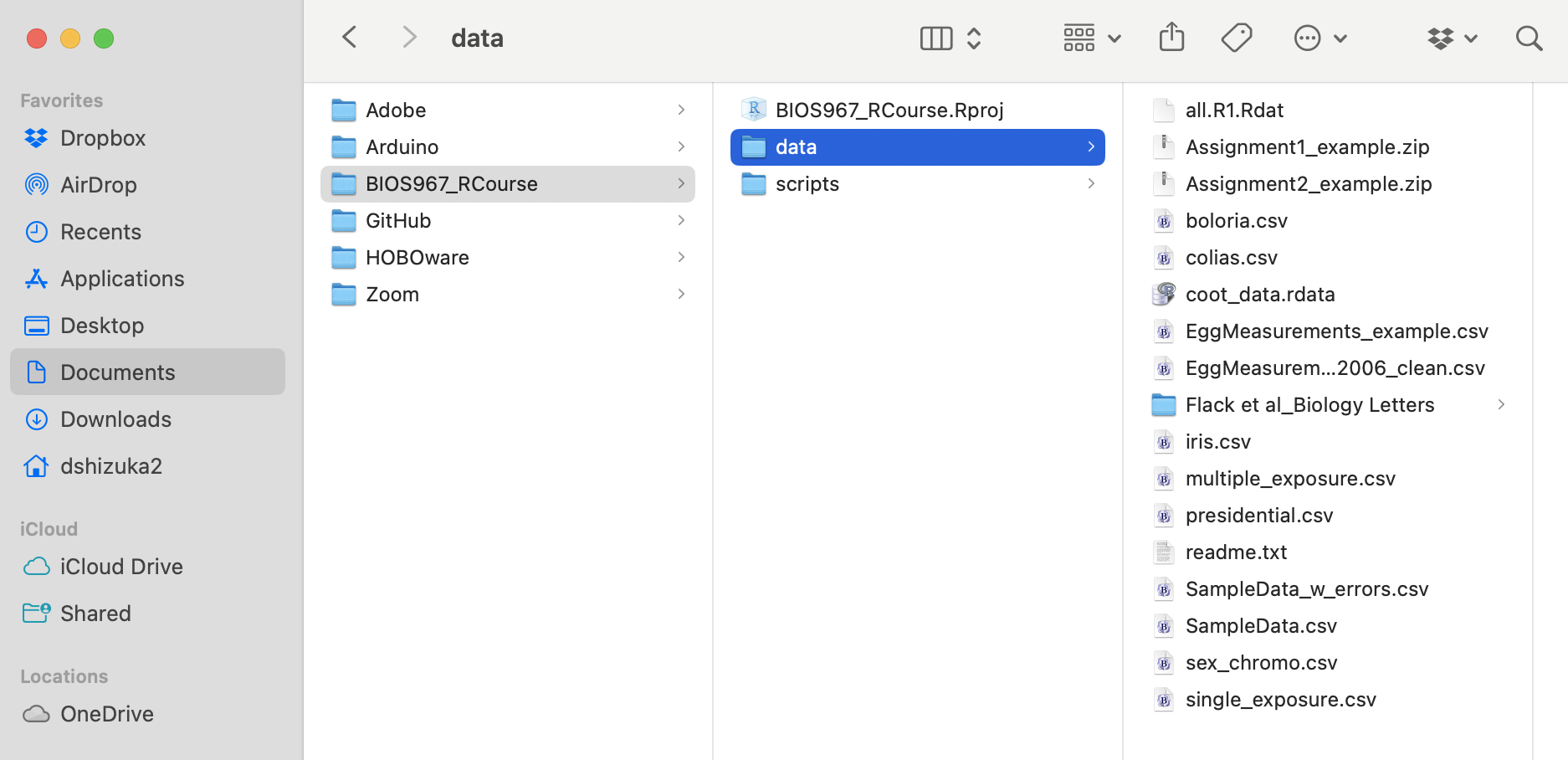
2.1 Importing a .csv file
In this case, my data files are inside a subfolder called “data”. So
the pathname is data/SampleData.csv Using this, I can read
in the .csv file using a function called read.csv(), with
the path name. Note that the path name needs to be inside
quotes.
dat=read.csv("data/SampleData.csv")2.2 importing from .txt file or other text-based file formats.
R is very good at importing from .txt files or anyt other text-based file formats. You just need to make sure you know the format–i.e., whether there are headers or other lines of text at the top, what kind of delimitation is used (e.g., comma-delimited vs. tab-delimited vs. space-delimited, etc.). In fact, if you know how to work with these options, it allows you to work with an even wider array of data.
A more generic function is read.table(). This function
allows you to read any kind of text file (including .csv files) while
specifying the data is delimited. So, for example, you can use this
function to import comma-separated files
dat=read.table(file.choose(), sep=","), or tab-delimited
files dat=read.table(file.choose(), sep="\t"). So the
read.table() function is more flexible in many ways.
2.3 Loading a .rdata file.
In R, you also have the option of “loading” an .rdata file format, which is a binary file format used by the R programming language. .Rdata files can store multiple objects together. This is a super useful way to share data.
load("data/coot_data.rdata")You should see that three datasets appeared in your “global environment”: “chick_color”, “chicks”, and “eggs”. These are three datasets associated with a worked example module on coot chick colors
3. The Not recommended ways to import data, and why I don’t recommend them.
3.1 Entering the full path name
You can also use the full path name to import the data. This might be helpful if you are not using Rstudio Projects and/or saving your script in a folder separate from your data.
Finding the path to a file Here is how to get the path to the .csv file on your computer.
- For Windows, you can get the path name of the file or folder by right-clicking it and click “Copy as Path”
- For Mac (or Windows), you can look for the file/folder in Finder, and then drag and drop the icon into the “Go to file/function” bar at the top of the RStudio window.
As an example, say I made folder on my desktop
called Rcourse and inside that folder, I made another
folder called Week_2. If my data folder is inside that,
this would be the path:
/Users/dshizuka/Desktop/Rcourse/Week_2/data
In turn, the path to a file inside that folder might be:
/Users/dshizuka/Desktop/Rcourse/Week_2/data/SampleData.csv
So in this case, your line of code to import the data would be:
dat=read.csv("/Users/dshizuka/Desktop/Rcourse/Week_2/data/SampleData.csv")Alternatively, you can use
setwd() to set your working directory, and then enter a
simpler path name. This essentially breaks up the process into two
lines:
setwd("/Users/dshizuka/Desktop/Rcourse/Week_2")
dat=read.csv("data/SampleData.csv")
Remember: You will have to change the path inside the lines of code here to be where the file resides in your computer.
Why using the absolute pathname is not recommended:
This option works fine as long as you are only ever working on code on one computer (and you never move your data file). But as soon as you try to run this same code on a different computer, it will fail. You will have to find the absolute pathname for the data file on that particular computer and then edit the code. This might not be something you encounter very often when you are working on one thesis/dissertation project on your own–but it will matter a lot as soon as you are trying to seek help from others on code development, or if you are collaborating on a project with someone because your code is only reproducible on your computer. So be nice to your future self–make it a routine to establish an RStudio project.
3.2 Use a url (good for data downloadable from the web)
Sometimes, you will be downloading a dataset that is accessible online, from a static website, a github page, a data repository (like Dryad or Figshare), or even a dropbox folder. In fact, if you can get a url of a data file, you can import it directly into R without having to first downloading it to your computer, saving it and then getting a path name.
For example, if you right-click on the link up above to download the
“SampleData.csv” file (under 3.1: Importing Data), you can “copy link
address” and get this url:
https://dshizuka.github.io/RCourse/data/SampleData.csv
So, you can simply download that file using this url instead of the path name:
dat=read.csv("https://dshizuka.github.io/RCourse/data/SampleData.csv")Why using url is not recommended:
Honestly, this method is super useful when it works! But note: only use this if you know that the url is going to be stable for a long time! If you need to be able to reproduce your analysis in the long term, it will probably pay off to download the data and save it on your computer and set up an RStudio project folder.
3.3 Call ‘choose file’ prompt.
You can also call a prompt that will let you choose the file. You can then find and choose the file you want to import. This is a convenient and quick way to import data. However, it is limiting because it takes time to click around to find the file, and more importantly, this step is not reproducible.
dat=read.csv(file.choose())3.4 Using RStudio GUI
In RStudio, select
[File]–[Import Dataset]–[From CSV...]
The first time you do this, you may be asked to install the
readr package.
Why using the ‘choose.file()’ prompt or the GUI are not recommended:
These methods defeat some of the main purpose of using code! First, when you have to click around to find your file, it takes time each time you are running the code. Importantly, this procedure is not as reproducible as code–when you embed the code to import the data properly, you ensure that anyone trying to run the code will get it right. Also, it is too easy to forget which version of the dataset you are supposed to be using, and you can make mistakes. You can prevent all that by just writing the code to import the data.
3.5 Reading straight from .xls or .xlsx
Ok, I will admit to you that there are times when it is just easier to write code to import directly from the default Excel format (.xls or .xlsx). For example, if you have to constantly update your data, it feels inconvenient to have to constantly remember to convert it into .csv format. You may also have to import a whole batch of data that are already saved as Excel sheets, and you don’t want to go through the trouble of converting each of them to .csv…
Whatever the reason, it IS possible to import data straight from Excel formats by using other R packages.
To use a function in a package, you have to first make sure that the
package is downloaded to your computer. The
install.packages() function downloads the package from an
online repository to your computer.
install.packages("readxl")But to USE the package in your current R environment, you have to
load the package. You can do that using either library() or
require(). They both work–if you want to know the
difference, just do a web search for “what’s the difference between
library and require in R?”
library(readxl)Now, you can use the read_excel() function to download
an .xlsx version of the SampleData file:
dat_xlsx=read_excel("data/SampleData.xlsx")

dat_xlsx
## # A tibble: 13 × 6
## `Individual ID` sex age size weight `date captured`
## <chr> <chr> <chr> <dbl> <dbl> <dttm>
## 1 20-01 male adult 29.5 66.5 2001-05-04 00:00:00
## 2 20-02 male juvenile 28 58.5 2001-05-05 00:00:00
## 3 20-03 female adult 26 57 2001-05-10 00:00:00
## 4 20-04 female adult 25 55.5 2001-05-10 00:00:00
## 5 20-05 female juvenile 25 62 2001-05-10 00:00:00
## 6 20-06 male juvenile 28 61 2001-05-12 00:00:00
## 7 20-07 female adult 26 58 2001-05-13 00:00:00
## 8 20-08 male adult 28.5 65 2001-05-13 00:00:00
## 9 20-09 male juvenile 27.5 60 2001-05-13 00:00:00
## 10 20-10 female juvenile 26 59 2001-05-13 00:00:00
## 11 20-11 male adult 25.5 62 2001-05-15 00:00:00
## 12 20-12 female adult 27 59 2001-05-16 00:00:00
## 13 20-13 female adult 26.5 60 2001-05-16 00:00:00You might notice that this output is formatted slightly differently than data frames you’ve seen before. It is called a ‘tibble’ format, which is used by the ‘tidyverse’ family of packages. You’ll learn more about that in the ggplot and data wrangling modules later on.
Why importing directly from .xlsx is less preferred:
Honestly, this method is not that bad, especially if you get used to it, so I do use this option sometimes. However, my main gripe with reading straight from .xlsx is that, in trying to be friendly, it makes formatting decisions that are not best practice for coding. For example, check the column names of this dataset:
names(dat_xlsx)## [1] "Individual ID" "sex" "age" "size"
## [5] "weight" "date captured"It includes column names that have spaces in them, like “Individual ID”. Now, try calling that column:
dat_xlsx$Individual IDYou will find that this code will not run–because you can’t have an object name that has a space. Instead, you have to use the “`” symbol around the column name to call it:
dat_xlsx$`Individual ID`## [1] "20-01" "20-02" "20-03" "20-04" "20-05" "20-06" "20-07" "20-08" "20-09"
## [10] "20-10" "20-11" "20-12" "20-13"This might seem like small details, but it CAN cause a lot of headaches downstream. Also, there is the basic problem of proprietary file formats. If you truly want to use open science practices, you should avoid sharing data and code using .xlsx format because computers that don’t have Microsoft Office cannot open them.
4. Looking at the data
Now that you have the data imported as an object called
dat, let’s look at it! You can do this simply by calling
the object:
dat## Individual.ID sex age size weight date.captured
## 1 20-01 male adult 29.5 66.5 5/4/01
## 2 20-02 male juvenile 28.0 58.5 5/5/01
## 3 20-03 female adult 26.0 57.0 5/10/01
## 4 20-04 female adult 25.0 55.5 5/10/01
## 5 20-05 female juvenile 25.0 62.0 5/10/01
## 6 20-06 male juvenile 28.0 61.0 5/12/01
## 7 20-07 female adult 26.0 58.0 5/13/01
## 8 20-08 male adult 28.5 65.0 5/13/01
## 9 20-09 male juvenile 27.5 60.0 5/13/01
## 10 20-10 female juvenile 26.0 59.0 5/13/01
## 11 20-11 male adult 25.5 62.0 5/15/01
## 12 20-12 female adult 27.0 59.0 5/16/01
## 13 20-13 female adult 26.5 60.0 5/16/01This data only has 13 rows, so it’s manageable. But sometimes you
have a much larger dataset, and you don’t really want to see all of it,
but you want to check that the correct data was imported. In that case,
you can use a function called head() which will show you
just the first 6 lines of an object.
head(dat)## Individual.ID sex age size weight date.captured
## 1 20-01 male adult 29.5 66.5 5/4/01
## 2 20-02 male juvenile 28.0 58.5 5/5/01
## 3 20-03 female adult 26.0 57.0 5/10/01
## 4 20-04 female adult 25.0 55.5 5/10/01
## 5 20-05 female juvenile 25.0 62.0 5/10/01
## 6 20-06 male juvenile 28.0 61.0 5/12/01You can also use the str() function to get the structure
of the data frame, including summary stats for numeric variables:
str(dat)## 'data.frame': 13 obs. of 6 variables:
## $ Individual.ID: chr "20-01" "20-02" "20-03" "20-04" ...
## $ sex : chr "male" "male" "female" "female" ...
## $ age : chr "adult" "juvenile" "adult" "adult" ...
## $ size : num 29.5 28 26 25 25 28 26 28.5 27.5 26 ...
## $ weight : num 66.5 58.5 57 55.5 62 61 58 65 60 59 ...
## $ date.captured: chr "5/4/01" "5/5/01" "5/10/01" "5/10/01" ...5. Formatting spreadsheets to keep data for analysis
This part is not necessarily about R. It is about managing your Excel sheet in a way that facilitates data analysis outside of Excel.
Before I start, I highly recommend this free online resource from datacarpentry.org: “Data Organization in Spreadsheets for Ecologists”
One of the reasons that many formatting problems arise while keeping data in spreadsheets is that the common software (e.g., Excel) is actually used for many different purposes. For example, people often use excel to generate templates for forms (e.g., purchasing forms). Best practices for those uses of Excel are completely different from what you should do when using spreadsheets for entering data.
Similarly, you might use spreadsheets with formatting for purposes other than keeping data for analysis (e.g., using it as a way to track progress on a project). The formatting for that kind of use is different than for storing data.
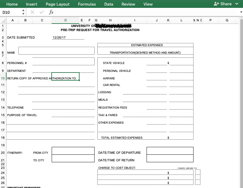
Spreadsheets are used for many different purposes, which explains many common formatting mistakes in data. This is a form made in Excel. NOT a good example of a data set.
5.1 Basic structure of a spreadsheet
First line (Header) are names of variables. Each variable is one column. Do not use values as column names.
Each subject (animal, plant, cell, etc.) should have an ID. This is useful if you have multiple spreadsheet where you have different information about the subject–if you have a common ID, you can link together datasets more easily.
Each row should be an observation. If you are observing a subject multiple times (e.g., repeated measures design), each observation should be a separate line, with the measurment time/place/trial/etc. as a separate column.
Don’t add totals on the last line of the data. Also, avoid calculating group averages, etc. to your data.
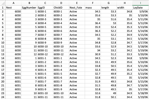
Example spreadsheet of data on egg size of American Coots
5.2 Spreadsheet dos and don’ts!
1. Don’t keep multiple tables in one sheet
This is one common way people have used excel sheets when your data comes from multiple sources (e.g., multiple plots). It also makes you feel like you have maximum information in the sheet. But in reality, this makes it impossible to do any global analysis. And R cannot read in this type of spreadsheet.
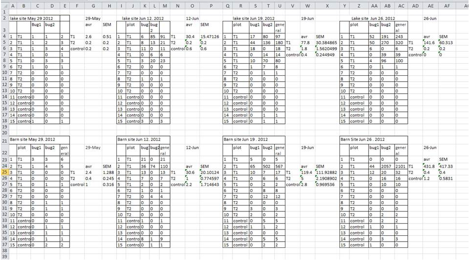
Solution: Just keep one sheet. If you have multiple plots, treatments, etc., make that a column in your data. Example in 4.1.1***
2. Don’t include title/metadata/table caption at the top (or bottom) of your data.
*The first row of your dataset should always be your column names (header). Don’t add extra information at the top of your dataset. If you need to add extra information about the data, put it in your readme file.
*Similarly, the last line of your dataset should be the last set of observations. Don’t include column totals/subtotals, etc. at the end of your dataset. This will cause problems when reading the data into R.
3. Don’t use special characters or commas.
Excel is capable of handling special characters that other software cannot. For example, if you have the ‘degree’ symbol (C\(^\circ\)) or ‘em dash’ (where “–” gets converted to one long dash), these will not be read correctly when you import data in R. Do NOT use these special characters in your data.
Also, commas cause problems when you are saving data in .csv files because the commas are designated for separating columns. If you like to write notes in your data, just make sure you don’t use commas! (e.g., if need be, you could use semi-colons)
Solution: Always think about whether your inputs will be read correctly by R or other stats program. Default to non-proprietary formats.
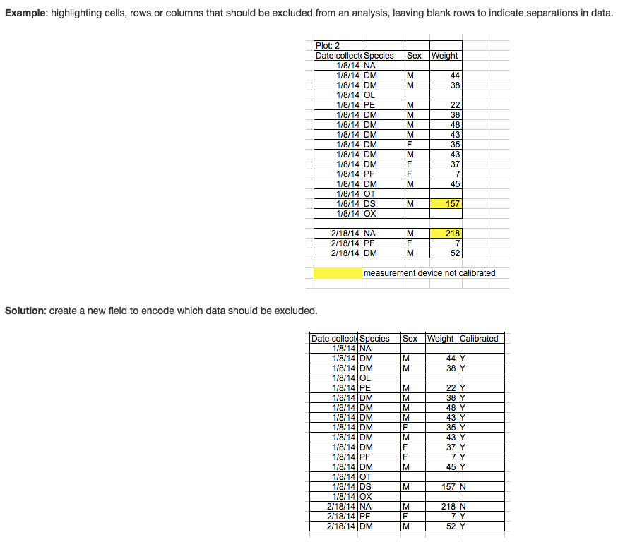
4. Don’t use formatting (i.e., highlighting) to convey information or make spreadsheets look pretty by merging cells.
This is a common mistake that comes from using Excel as forms.
If you are using highlighting to indicate some information, it you can almost always just add another column to include that information as another variable (see example figure). Merged cells will make R unable to import the file.
5. Do use good ‘null values’
Always put in 0 if the observed vaule is 0 (i.e., don’t skip the cell just because it’s 0). If you don’t it becomes indistinguishable from unknown or unobserved data.
Don’t use other numbers (e.g., 999 or -999). This used to be common practice for some stats software. But this can cause problems because it may be inadvertently used in calculations.
Don’t use other symbols (-, ., ?). Again, this used to be common practice for some people, but this can cause problems because R won’t know how to interpret it.
Good options include:
- Blank cells. But only if you are careful to always put 0 when the correct value is 0.
- Consistent, conventional abbreviation (e.g., NA, NULL). But note that “NA” may be used as abbreviations for other things, like “North America”. But if used in a column that is otherwise numeric, R can automatically interpret this as null value.
If you are using consistent null value designations, you can specify
these values as null using the na.string= argument within
the read.csv() function. For example,
dat=read.csv("data/SampleData.csv", na.string=c("NA", "#N/A"))The above code will tell R that cells with either “NA” or “#N/A” should be interpreted as missing data.
6. Do use good column names (variable names)
Avoid using special characters or spaces in your column names. These will automatically converted to “.” when you import to R. Removing spaces or using “_” or “.” instead will make your life easier.
Use relatively short but informative column names. But keep a readme.txt file associated with your data where you store detailed information on how each variable was measured.
7. Avoid keeping summary data along with raw data (i.e., don’t make a “group means” column in your dataset).
This is more of a suggestion than a rule. When you use formulas within Excel to calculate summary values, those formulas do not carry over when you convert the spreadsheet to .csv. This means that if you need to do any recalculations, or if you realize there are any errors in values, those summary values will become outdated. It is much easier (and better) to calculate summary values within R anyway.
Key rule in reproducible research: Try not to mess with raw data!
Once you have collected data, it is best to try to keep that raw data raw. If you find coding errors or you need to subset data for your analyses, it is best to do that with R once the data has been imported. This is because data-cleaning in R is reproducible. But once you start messing with raw data, it is way too easy to lose track of what you “fixed” and what you did not. Also, there are times when you later realize that you “fixed” the data incorrectly. If you have done all of that in excel, it is difficult to go back. But if you have done everything in script, everything is reversible.
6. Troubleshooting Data Import
Even when you have taken care to follow the above dos and don’ts, you will often have some kind of problem reading in files. One of the big roadblocks to using R is dealing with these bugs.
Some common problems:
- File won’t import
- Are you sure you saved the file as a .csv file?
- Is the path and file name correct?
- Is the path and file name inside quotes?
- I get a weird column that has a bunch of
NA- You probably have a column in your spreadsheet that has a value in one of the cells that you forgot about.
- I have a weird column at the bottom of my data that is just
a bunch of
NA- You probably have a cell at the bottom of your spreadsheet with “hidden spaces”.
- Fix: In excel, do a “Find and Replace” to replace blank space with some character (e.g., a *) and then go and find and erase those characters.
- Column is supposed to be numeric but it is showing up as
factors.
- You probably have a cell value in the column that is non-numeric, e.g., “#N/A” or ‘hidden space’
- Fix: You can specify what kind of characters should be interpreted
as
NAusing thena.string=argument (see above).
Group Exercise 1: Troubleshoot data import
Step 1: Import the SampleData_w_errors.csv file and look
at its data structure:
##    Indiv_ID    sex      age size weight  X
## 1     20-01   male    adult 29.5   66.5  1
## 2     20-02   male juvenile   28   58.5 NA
## 3     20-03 female    adult   26  #N/A! NA
## 4     20-04 female    adult   25   55.5 NA
## 5     20-05 female juvenile   25     62 NA
## 6     20-06   male juvenile   28     61 NA
## 7     20-07 female    adult   26     58 NA
## 8     20-08   male    adult 28.5     65 NA
## 9     20-09   male juvenile 27.5     60 NA
## 10    20-10 female juvenile   26     59 NA
## 11    20-11   male    adult 25.5     62 NA
## 12    20-12 female    adult   27     59 NA
## 13    20-13 female    adult 26.5     60 NA
## 14                            **        NA
Step 2: Fix the spreadsheet so that you get the following:
- The column called “sex” only has “female” and “male”.
- The column called “size” is numeric
- The column called “weight” is numeric
- The column called “X” is removed.
See how to fix these errors in R here
Group Exercise 2: Improve my egg measurement data
Find the dataset called “EggMeasurements_example.csv” in the data folder. This is real data I collected on egg sizes of American Coots (Fulica americana) before I knew anything about R or programming.
Try importing the data to R and also look at the spreadsheet in Excel.
Come up with as many recommendations as possible on how to improve this excel sheet.
See the answers here