Directories, Pathnames, and RStudio Projects
BIOS 967: Intro to R for Biologists
Dai Shizuka
updated 08/29/25
Note: You can get a lot of this information from Hadley Wickham’s “R for Data Science” book, Chapter 8: here.
Do this before you start this section!
- Click on the following link to download this file: SampleData.csv
- Save this file somewhere on your computer where you can find it.
1. What we are talking about here and why.
This module introduces the idea of organizing a workflow, which can involve importing data, generating (and saving) graphics, writing new data outputs, etc. Importantly, we want to do all of this without relying on pull-down menus or clicking buttons. Rather, we will do all of this by code. Why? Because code can be made to be reproducible–i.e., we can set up the code so that it works on any computer the same way. Thiw way, we can produce results that can be reproduced by anyone, every time, simply by running that code. On the other hand, button-clicks are not reproducible in the same way. Maybe you can re-create an entire routine of button-clicks by leaving yourself very detailed instructions… but leaving yourself reproducible code is much easier.
I admit that all of this will feel like it’s overly cumbersome at the beginning. But trust me, this is going to pay off very quickly. After learning how to setup your workflow, you will be able to share code, results, and troubleshoot with collaborators (including your ‘future self’) much faster and reliably. Importantly for this class, it will also help me help you better in your independent project, because I will be able to run your code, reproduce your errors, and help you find fixes.
To do all of this, we need to be able to talk to the computer about where to find files and where to put files. This seems like a basic thing, but it is often the biggest first hurdle in learning computer programming. The computer can’t think like you and intuit where the proper file might be, or where it should put it–it needs to be told explicitly.
Some terminology
directory: Essentially, this is a folder on your computer.
working directory: This is the directory (folder) that computer treats as the default place to look for files, or to write (save) output files.
pathname: A string of directory and file names that specifies exactly where on your computer the particular file is located.
absolute path: This is a string that specifies where a particular file is on your computer, starting from the root directory of your computer.
relative path: This is a string that specifies where a particular file is relative to your working directory (i.e., instead of the root of your computer).
3. Using Rstudio Projects and organizing your files.

Rstudio projects facilitate a important “best practice” for developing code to facilitate your research, which is to make sure that for each project, create one folder that contains all of your data, scripts, outputs (e.g., plots) and other assets.
Additionally, I highly recommend that this “project directory” folder includes a subfolder called “data” that contain all of the data files, and “figures” (or some other name) folder that will contain all of the output plots, etc.
Setting up a project directory in this way allows you to keep everything organized and up to date, and it also helps with collaborations or sharing code, because it is easy to follow where things are. It is also nice for your “future self”–if you come back to a project after some time, it is easy to pick up where you left off without wondering where you left all of the relevant files.
Finally, the more important reason to set up an Rstudio project folder is that it will allow anyone to run the code you are developing in this folder because you all of your pathnames will be “relative” to the parent directory. By using relative path names in your code, it becomes much more reproducible and enables collaboration.
Reading about all of this is one thing, but you’ll actually learn how this works by using it! So, let’s set up an RStudio Project directory that you will use for the rest of the lectures for this course. Please follow these directions and set up your folder exactly the same way, with exactly the same folder names (including capitalization).
3.1. Setting up a new Rstudio project folder the course lectures.
Create a folder called “BIOS967_RCourse” on your computer.
Next, in R Studio, click on “File” > “New Project”
Click on “Existing Directory”, click “Browse” and select the “BIOS967_RCourse” Folder you created, then click “Create Project”
Now, you will see that there is a new “BIOS967_RCourse.rproj” file in your folder.
Open that .rproj file. This will open up a new RStudio window.
Now, whenever you create any file within this R Project, the files will automatically go into this folder. Also, if you want to import any files, you can just put in the file name instead of the whole path.
- Create a “data” folder with all data needed for all learning modules.
Click on this link to download a compressed file with all data from the learning modules.
“Decompress” or “unzip” the file. This will create a folder called “data”. Move this folder into your “BIOS967_RCourse” folder.
Finally, create a second folder, called “scripts”. This is where you will store code scripts.
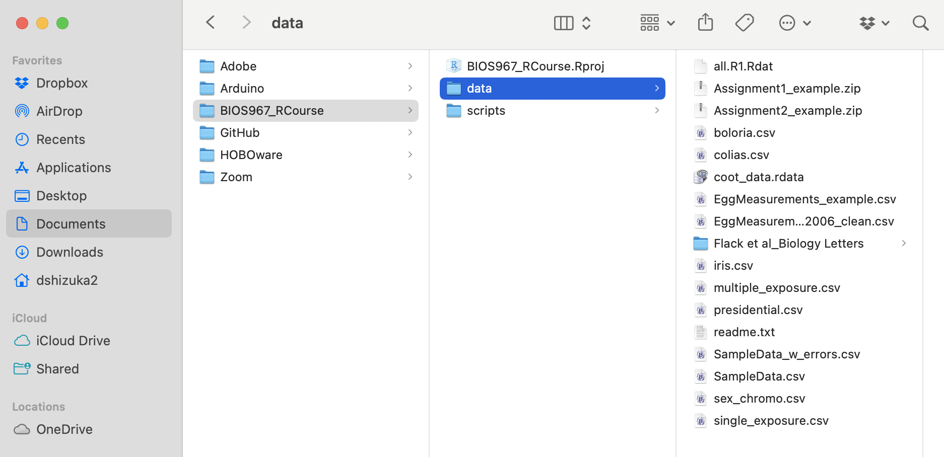
Now, in RStudio, click on the “refresh” button
 on the far right side of your
“Files” window on the bottom-right part of your Rstudio window. You
should now see the “data” and “script” folders in your project
directory, and there should be bunch of files in the “data”
folder.
on the far right side of your
“Files” window on the bottom-right part of your Rstudio window. You
should now see the “data” and “script” folders in your project
directory, and there should be bunch of files in the “data”
folder.
4. What you will do from now on:
Now that we have created the proper file structure for this project folder for the lectures in this course, here is the workflow from now on: Always start by opening the “.rproj” file.
This starts an R session with the working directory set to the folder where the .rproj file resides.
What does this mean?
First, it means that you don’t need to use absolute pathnames any
more–you just need the relative pathname. For example, to import the
“SampleData.csv” data, you only need to put in
"data/SampleData.csv" to tell R to look for
“SampleData.csv” inside the “data” folder, instead of the whole pathname
on your computer.
Let’s call this version of the data dat2
dat2=read.csv("data/SampleData.csv")dat2## Individual.ID sex age size weight date.captured
## 1 20-01 male adult 29.5 66.5 5/4/01
## 2 20-02 male juvenile 28.0 58.5 5/5/01
## 3 20-03 female adult 26.0 57.0 5/10/01
## 4 20-04 female adult 25.0 55.5 5/10/01
## 5 20-05 female juvenile 25.0 62.0 5/10/01
## 6 20-06 male juvenile 28.0 61.0 5/12/01
## 7 20-07 female adult 26.0 58.0 5/13/01
## 8 20-08 male adult 28.5 65.0 5/13/01
## 9 20-09 male juvenile 27.5 60.0 5/13/01
## 10 20-10 female juvenile 26.0 59.0 5/13/01
## 11 20-11 male adult 25.5 62.0 5/15/01
## 12 20-12 female adult 27.0 59.0 5/16/01
## 13 20-13 female adult 26.5 60.0 5/16/01This will also simplify the process of saving files and plots–which we will do later.
The beauty of this system is that, as long as the project directory structure is the same the computer, you can run this exact same code to import the data on any computer. In turn, that means that this entire project and code are portable in multiple ways. You could:
send a collaborator your whole project directory, or
copy the project directory on a thumbdrive, or
sync the project directory on DropBox, OneDrive, or other cloud storage that syncs with multiple computers…
or, the best way–make this project folder into a GitHub repository (or other Git system), where you and collaborators can keep the project folder synchronized as you work. In class, we will do this together later to setup repositories for your independent projects. To learn how to do this, go to the “GitHub Workflow” module.