Packages you will need for this tutorial:
library(igraph)
One of the assumptions of network theory is that the connections
between elements in a system matter to the function/property of the
system and/or the individual elements within the system. One way in
which such connections matters is that they can facilitate the flow of
something through this system. Some examples include:
- Electricity through an electric grid
- Bits of information through the internet
- Vehicles/individuals moving through a transportation network
- Information through social networks
- Disease through contact networks
- Modification of social strategies through competition networks
One of the classical theories on social spread is that the
accumulation of individuals (nodes) that take on a new state (e.g., an
innovation) takes on different pattern when the spread is due to asocial
processes (e.g., everyone innovates on their own) versus social
processes (e.g., innovation spreads through social transmission).
Here, let’s explore this paradigm by actually simulating the spread
of innovation due to asocial or social processes.
8.1 Simulation of asocial changes in state (e.g., asocial
learning)
Let’s first consider a situation where each individual in a social
network has an inherent probability to adopt the innovation at any given
time.
First, we will make a random graph consisting of 100 nodes. We will
set the initial ‘innovation adoption’ status for all individuals (all
initially 0).
set.seed(4)
n=100
g=erdos.renyi.game(n, p=0.05)
V(g)$status=0 #the 'innovation adoption status' for each individual. All initially 0.
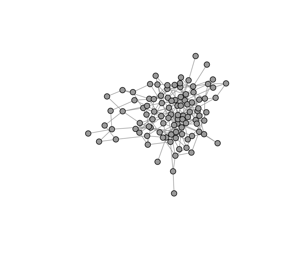
Let’s plot this random graph. While we’re at it, we will save the
layout so that we can use it for all the plots of this network
later.
l=layout_with_fr(g)
plot(g, vertex.label="", vertex.size=8, vertex.color="darkgray", layout=l)

Now, we will set the ‘asocial learning’ parameter, \(x\) to be 0.1. This is the probability that
any given individual will come up with the innovation–e.g., how to
forage for a new prey item.
x=0.1
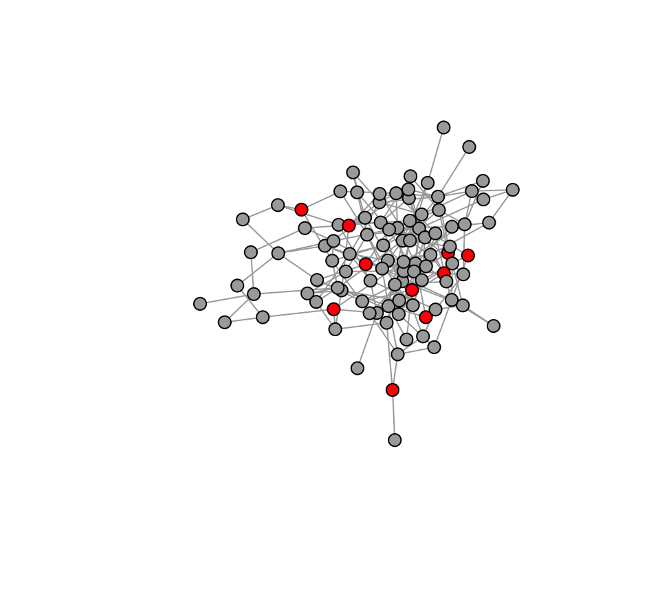
Let’s run one practice run of how this will work. In one time step,
we flip a coin for each individual whether or not they will adopt the
innovation. Based on the coin flip, we will convert the status of the
individual to 1 if they learned the innovation in that time step:
naive=which(V(g)$status==0) #which individuals have not adopted yet?

adopt=sample(c(1,0), length(naive), prob=c(x, 1-x), replace=T) #based on the probabilities, flip a coin for each naive individual and determine if the individual adopts the innovation in the current time step

V(g)$status[naive][which(adopt==1)]=1 #change status of individuals whose status is 0 and is in the list of new adopters

plot(g, vertex.label="", vertex.color=c("darkgray", "red")[V(g)$status+1], vertex.size=8, layout=l)

Now, we will repeat this simulation for 30 time steps. Here, we need
to consider that any given individual can only adopt an innovation once
(it can’t go back). If you’re thinking about this in terms of disease,
it’s like an ‘SI model’ in which individuals do not recover or go back
to a susceptible state. In practical terms, this means that we will just
ignore coin flips for individuals whose status = 1.
t=30
g.time=list()
V(g)$status=0
for(j in 1:t){
  naive=which(V(g)$status==0)
  adopt=sample(c(1,0), length(naive), prob=c(x, 1-x), replace=T)
  V(g)$status[naive][which(adopt==1)]=1
  g.time[[j]]=g
}
What we end up with is 20 igraph objects in a list called
g.time (output not shown)
g.time
In these graphs, the only thing that changes across these 20 times
steps is the individual status. In each time step, there will be more
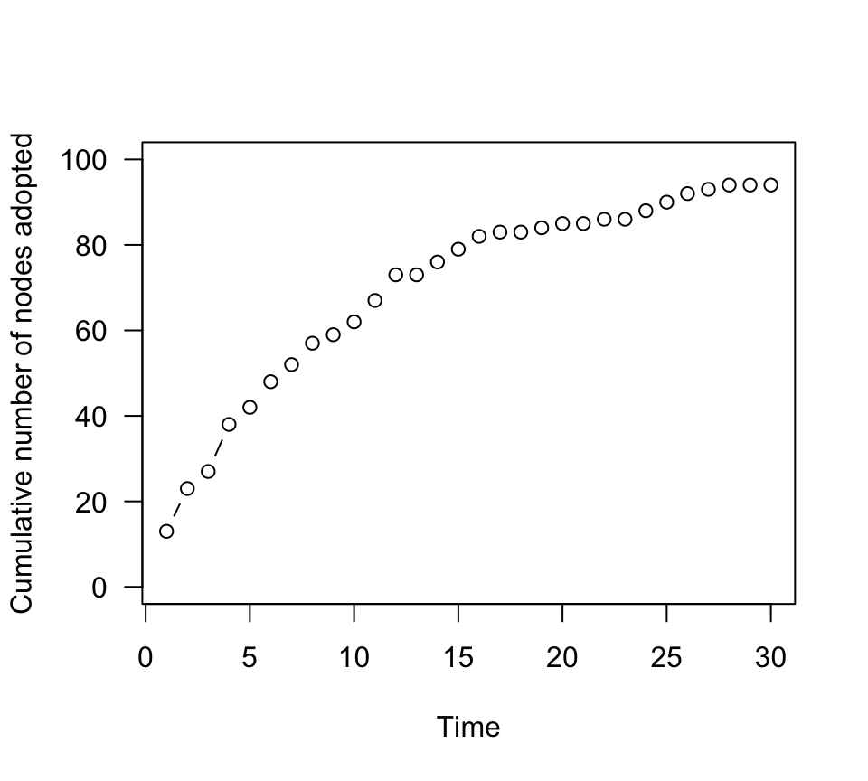
individuals that adopt the innovation. We can plot how many cumulative
individuals adopt the new innovation (i.e., become status=1) across time
steps:
n.adopt.asocial=sapply(g.time, function(x) length(which(V(x)$status==1))) #for each time step, count the number of individuals that have adopted the innovation
plot(n.adopt.asocial, type="b", las=1, ylab="Cumulative number of nodes adopted", xlab="Time", ylim=c(0,100))

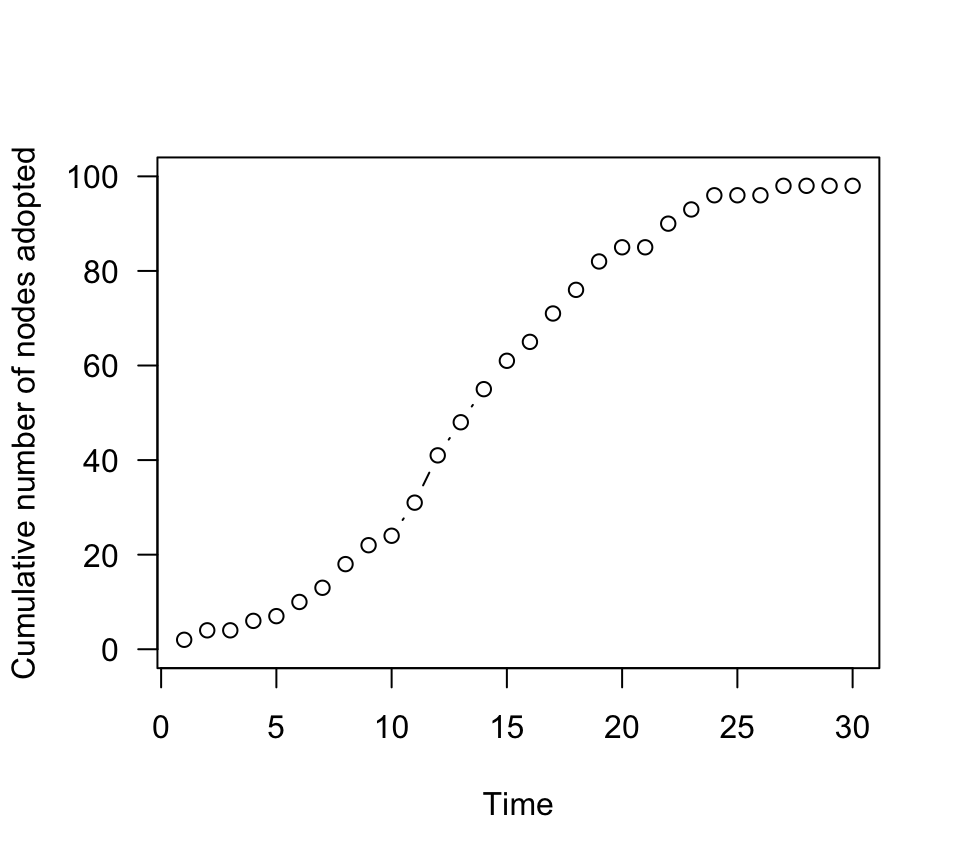
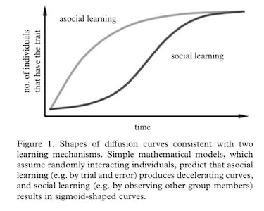
You should see that, in the asocial learning case, there is a
decelerating accumulation curve of individuals that adopt the
innovation. This is because all individual have the same probability of
adopting the new status at any given point, but they never go back–so
there are fewer individuals left that hasn’t adopted the innovation as
time goes on. Thus, there is a steady decelerating rate of adoption of
the innovation.
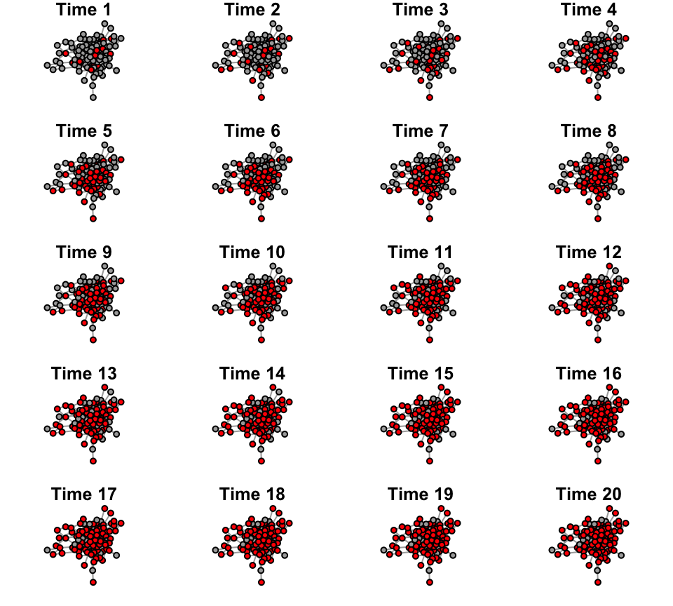
For visualization purposes, let’s plot the network across the first
20 time points.
def.par <- par(no.readonly = TRUE)
layout(matrix(1:20, byrow=T, nrow=5))
par(mar=c(1,1,1,1))
for(i in 1:20){
  v.col=c("darkgray", "red")[V(g.time[[i]])$status+1]
  plot(g.time[[i]], vertex.label="", vertex.color=v.col, layout=l, main=paste("Time",i))
}

8.2 Simulation the social transmission of whatever state in
a random graph
Now, let’s take the same network and try the case where a new
innovation spreads socially. That is, an innovation is socially
transmitted.
First, we’ll start over by creating a graph object, but we’ll use the
same set.seed() function so we can re-create the
connectivity of the asocial case.
set.seed(4)
n=100
g2=erdos.renyi.game(n, p=0.05)
l2=layout_with_fr(g2)
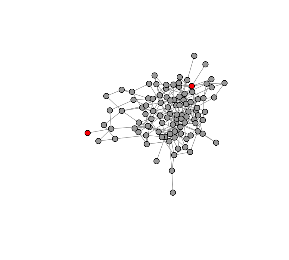
Next, we will create the “status” vertex attribute. Everyone will
start with state = 0. Then, we will randomly pick 2 nodes who will have
state = 1
V(g2)$status=0 # Create a vertex attribute for adoption status. 1 if the node has adopted the innovation. 0 if not.
seed=sample(V(g2),2) #select 2 innovators
V(g2)$status[seed]=1 #These 'seed' individuals get a status of 1 at the beginning.
plot(g2, vertex.label="", vertex.size=8, vertex.color=c("darkgray", "red")[V(g2)$status+1], layout=l2)

Now, we will set a “social transmission” parameter, \(s\). You can think of this as the linear
increase in the probability that an individual will take on a new
“state” (e.g., learn a new foraging strategy or get infected by a
disease) when it has a ‘neighbor’ that has that state. Since it’s a
probabilty 0 ≤ \(s\) ≤ 1.
Let’s set \(\tau = 0.1\) for
now:
tau = 0.1
Now we will simulate 30 time steps of the spread of this innovation.
We will save the network for each time point. The for-loop routine will
be as follows:
- first, we will use the
neighbors() function to identify
the neighbors (i.e., nodes connected to) of each node. We will use this
to add up the status of each node’s neighbors.
- Next, we will implement a social learning process in which the
probability \(p\) that an individual
that has not yet adopted the innovation will adopt in that time step =
\(1-e^{-\tau*s}\), where \(\tau\) is the parameter that describes the
influence of social learning, and \(s\)
is the number of neighbors of an individual that has already adopted the
innovation.
- Based on the calculated probability \(p\) for each individual, we then use the
sample() function to “flip a biased coin” to see if the
focal individual adopts the innovation or not.We do this for every
individual that has not yet adopted the innovation (i.e., status = 0).
Note that if the focal individual has already adopted the innovation,
then we just ignore that individual and move on.
- We then change the status of each individual that got a “1” in the
coin flip to status=1
- Return to step 1.
t=30 #time steps to run the simulation
g2.time=list() #empty list to store the output networks
for(j in 1:t){
  nei.adopt=sapply(V(g2), function(x) sum(V(g2)$status[neighbors(g2,x)]))
  p=(1-exp(-tau*nei.adopt))*abs(V(g2)$status-1) #here, we multiply the probabilities by 0 if node is already adopted, and 1 if not yet adopted
  adopters=sapply(p, function(x) sample(c(1,0), 1, prob=c(x, 1-x)))
  V(g2)$status[which(adopters==1)]=1
  g2.time[[j]]=g2
}
After this simulation has run, we will plot the accumulation curve
for the number of individuals that adopted the innovation through social
learning.
n.adopt.social=sapply(g2.time, function(x) length(which(V(x)$status==1))) #for each time step, count the number of adopters.

plot(n.adopt.social, type="b", las=1, ylab="Cumulative number of nodes adopted", xlab="Time", ylim=c(0,100))

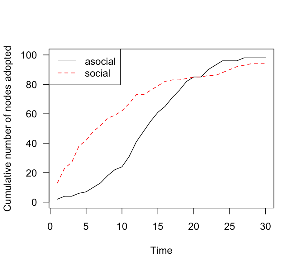
Ok, this accumulation curve looks different than the asocial case,
right? This is a clear “S-shaped” curve characteristic of social
learning. Let’s plot both the asocial and social case together:
plot(n.adopt.social, type="l", lty=1, col="black",las=1, ylab="Cumulative number of nodes adopted", xlab="Time", ylim=c(0,100))
points(n.adopt.asocial, type="l", las=1, lty=2, col="red")
legend("topleft", lty=c(1,2), col=c("black", "red"), legend=c("asocial", "social"))

This looks an awful lot like the theoretical expectation:
8.3 Animating social transmission using GIFs
Now, we will use the results of the simulations in section 11.2 and
animate the dynamics of social diffusion on a network.
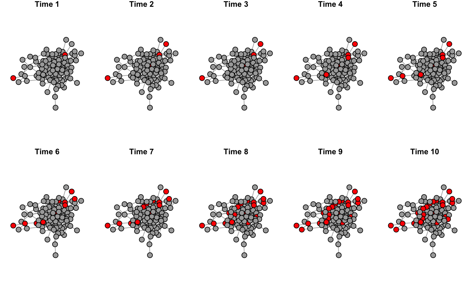
Let’s first try to plot what the network should look like for the
first 12 time points.
layout(matrix(1:10, byrow=T, nrow=2))
par(mar=c(1,1,1,1))
for(i in 1:10){
  v.col=c("darkgray", "red")[V(g2.time[[i]])$status+1]
  plot(g2.time[[i]], vertex.label="", vertex.color=v.col, layout=l2, main=paste("Time",i))
}

par(def.par)
What we are looking for here is to make sure that the network is laid
out identically in each panel, and only the node colors change as more
individual change status through social transmission.
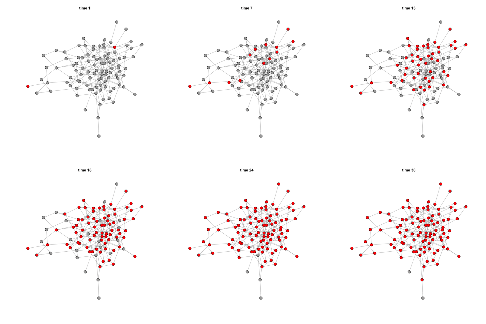
Ok, now we are ready to make a GIF that animates the change in the
social network across time. To do this, we will use the function
saveGIF() in the package animation. How this
function works is that you will run a for loop inside the function to
generate a batch of images that you want to stitch together as an
animation. Here is the code:
library(animation)

saveGIF(
  {for (i in 1:30) {
  plot(g2.time[[i]], layout=l2, vertex.label="", vertex.size=5, vertex.color=c("darkgray", "red")[V(g2.time[[i]])$status+1], main=paste("time",i,sep=" "))
  }
  }, movie.name="sample_diffusion.gif", interval=0.2, nmax=30, ani.width=600, ani.height=600)
When you run this code, the GIF file should actually pop up on your
screen. You can simply drag it to a web browser to see the animation. It
should look like this:

The speed of the animation can be set using the argument
interval=. Other arguments can be found by going to
?ani.options.
8.4 Effect of network structure on transmission dynamics
Shah et al. (2017) effectively showed how the structure of networks
influences transmission dynamics on networks. Here, we can play around
with the modularity of the social network and observe its effects.
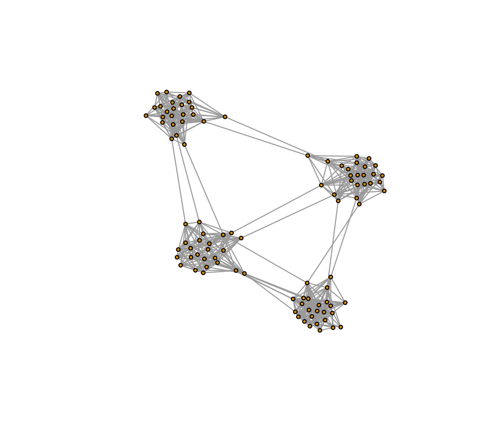
Let’s start with making a network of 100 nodes with strong community
structure. I’m going to assign 25 nodes each to four communities, and
then set the probability of edges to be much higher within communities
(0.5) compared to across communities (0.005)
set.seed(2)
n=100
mod.assign=c(rep(1,25), rep(2,25), rep(3,25), rep(4,25))
same.mod=outer(mod.assign, mod.assign, FUN="==")
p.mat=apply(same.mod, c(1,2), function(x) c(0.005, 0.5)[x+1])
adj=apply(p.mat, c(1,2), function(x) sample(c(1,0), 1, prob=c(x, 1-x)))
adj[lower.tri(adj)]=0
diag(adj)=0
adj=adj+t(adj)
g3=graph_from_adjacency_matrix(adj, "undirected")
l3=layout_with_fr(g3)
plot(g3, vertex.label="", vertex.size=3, layout=l3)
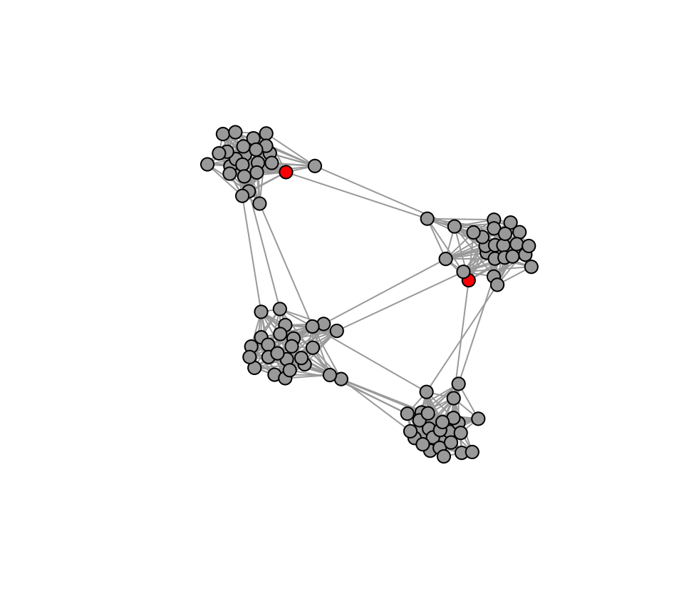
Then, we’ll select two random innovators.
V(g3)$status=0 # Create a vertex attribute for adoption status. 1 if the node has adopted the innovation. 0 if not.
seed=sample(V(g3),2) #select 2 innovators
V(g3)$status[seed]=1 #These 'seed' individuals get a status of 1 at the beginning.
plot(g3, vertex.label="", vertex.size=8, vertex.color=c("darkgray", "red")[V(g3)$status+1], layout=l3)
We’ll then run the simulation with the same tau parameter.
tau = 0.1
t=30 #time steps to run the simulation
g3.time=list() #empty list to store the output networks
for(j in 1:t){
  nei.adopt=sapply(V(g3), function(x) sum(V(g3)$status[neighbors(g3,x)]))
  p=(1-exp(-tau*nei.adopt))*abs(V(g3)$status-1) #here, we multiply the probabilities by 0 if node is already adopted, and 1 if not yet adopted
  adopters=sapply(p, function(x) sample(c(1,0), 1, prob=c(x, 1-x)))
  V(g3)$status[which(adopters==1)]=1
  g3.time[[j]]=g3
}
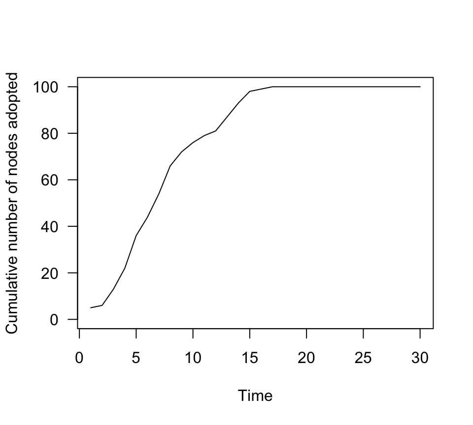
When we look at the transmission dynamics, we see that there is
faster spread overall.
n.adopt.social=sapply(g3.time, function(x) length(which(V(x)$status==1))) #for each time step, count the number of adopters.

plot(n.adopt.social, type="l", las=1, ylab="Cumulative number of nodes adopted", xlab="Time", ylim=c(0,100))
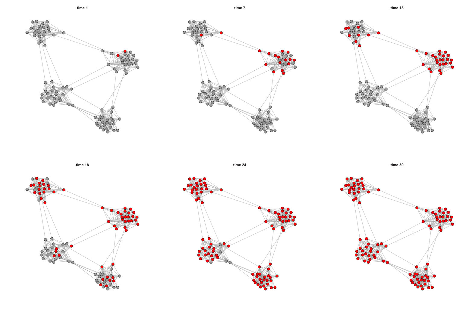
 But if we animate the network, we can see that the spread is highly
influenced by community structure.
library(animation)

saveGIF(
  {for (i in 1:30) {
  plot(g3.time[[i]], layout=l3, vertex.label="", vertex.size=5, vertex.color=c("darkgray", "red")[V(g3.time[[i]])$status+1], main=paste("time",i,sep=" "))
  }
  }, movie.name="sample_diffusion2.gif", interval=0.2, nmax=30, ani.width=600, ani.height=600)

8.5 NBDA: Network-Based Diffusion Analysis
Network-based Diffusion Analysis (NBDA) is a modelling approach to
ask the question, does the order or timing of acquisition of a behavior
or change state of an individual indicative of diffusion on a network?
NBDA does this through maximum likelihood model fitting. See Franz et
al. (2011), Hoppitt et al. () and Hasenjager et al. (2021) for details
on how this method works.
Here is a demo of NBDA on the social spread through the modular
network.
library(NBDA)
adj.mat=as_adj(g3, sparse=F)
adj.array=array(dim=c(nrow(adj.mat), ncol(adj.mat), 1))
adj.array[,,1]=adj.mat
#get list of individuals that solved at each time
solve.mat=sapply(g3.time, function(x){
  V(x)$status
})

#time of acquisition
ta=apply(solve.mat, 1, function(x) min(which(x==1)))
ta[is.infinite(ta)]=30
#order of acquisition
oa=order(ta)

diffdat=nbdaData("try1",  assMatrix=adj.array, orderAcq=oa, timeAcq=ta)

# oa.fit_social=oadaFit(diffdat, type="social")
# oa.fit_social@outputPar
# oa.fit_social@aic
# data.frame(Variable=oa.fit_social@varNames,MLE=oa.fit_social@outputPar,SE=oa.fit_social@se)

ta.fit_social=tadaFit(diffdat, type="social")
#ta.fit_social@outputPar
data.frame(Variable=ta.fit_social@varNames,MLE=round(ta.fit_social@outputPar,3),SE=round(ta.fit_social@se,3))
##                  Variable     MLE      SE
## 1         Scale (1/rate): 603.449 603.234
## 2 1 Social transmission 1 101.839 102.600
… as opposed to the case of asocial learning presented in section
8.1
adj.mat=as_adj(g, sparse=F)
adj.array=array(dim=c(nrow(adj.mat), ncol(adj.mat), 1))
adj.array[,,1]=adj.mat
#get list of individuals that solved at each time
solve.mat=sapply(g.time, function(x){
  V(x)$status
})

#time of acquisition
ta=apply(solve.mat, 1, function(x) which.max(x==1))
ta[is.infinite(ta)]=30
#order of acquisition
oa=order(ta)

diffdat=nbdaData("try1",  assMatrix=adj.array, orderAcq=oa, timeAcq=ta)

# oa.fit_social=oadaFit(diffdat, type="social")
# oa.fit_social@outputPar
# oa.fit_social@aic
# data.frame(Variable=oa.fit_social@varNames,MLE=oa.fit_social@outputPar,SE=oa.fit_social@se)

ta.fit_social2=tadaFit(diffdat, type="social")
#ta.fit_social2@outputPar
data.frame(Variable=ta.fit_social2@varNames,MLE=round(ta.fit_social2@outputPar,3),SE=ta.fit_social2@se)
##                  Variable   MLE  SE
## 1         Scale (1/rate): 0.000 NaN
## 2 1 Social transmission 1 9.744 NaN
##Next: 9. Random Graphs


 But if we animate the network, we can see that the spread is highly
influenced by community structure.