Worked Example: Wrangling World Bank Population Data

Things you will learn in this Worked Example

Practice wrangling data with dplyr and tidyr
Learn tricks to download data from public data repositories like the World Bank
More practice with ggplot
A little bit of stats

We will accomplish these while exploring the (admittedly superficial) patterns in population growth rates across countries.

By the end, you’ll be able to produce graphs like this:

Set up: load packages

library(wbstats)
library(tidyverse)

1. The Data: Population growth trends across the world

The World Bank actually makes it very easy to download a huge amount of data very easily. You could just go to the World Bankd Open Data site and search for data and download them in a few clicks. There are even packages such as WDI and wbstats that allow you to query and pull data from this site from within R.

However, for the purposes of this exercise, we will deal with several datasets that are included in the packages we have loaded above.

`world_bank_pop`: Population data from World Bank (2000-2017)

First is the world_bank_pop dataset that is included in the tidyr package (which is part of the the tidyverse suite). Start by pulling up the help file for the dataset

?world_bank_pop

Let’s take a peak at the data, which is in “tibble” format:

world_bank_pop

## # A tibble: 1,064 × 20
##    country indicator      `2000`  `2001`  `2002`  `2003`  `2004`  `2005`  `2006`
##    <chr>   <chr>           <dbl>   <dbl>   <dbl>   <dbl>   <dbl>   <dbl>   <dbl>
##  1 ABW     SP.URB.TOTL    4.16e4 4.20e+4 4.22e+4 4.23e+4 4.23e+4 4.24e+4 4.26e+4
##  2 ABW     SP.URB.GROW    1.66e0 9.56e-1 4.01e-1 1.97e-1 9.46e-2 1.94e-1 3.67e-1
##  3 ABW     SP.POP.TOTL    8.91e4 9.07e+4 9.18e+4 9.27e+4 9.35e+4 9.45e+4 9.56e+4
##  4 ABW     SP.POP.GROW    2.54e0 1.77e+0 1.19e+0 9.97e-1 9.01e-1 1.00e+0 1.18e+0
##  5 AFE     SP.URB.TOTL    1.16e8 1.20e+8 1.24e+8 1.29e+8 1.34e+8 1.39e+8 1.44e+8
##  6 AFE     SP.URB.GROW    3.60e0 3.66e+0 3.72e+0 3.71e+0 3.74e+0 3.81e+0 3.81e+0
##  7 AFE     SP.POP.TOTL    4.02e8 4.12e+8 4.23e+8 4.34e+8 4.45e+8 4.57e+8 4.70e+8
##  8 AFE     SP.POP.GROW    2.58e0 2.59e+0 2.61e+0 2.62e+0 2.64e+0 2.67e+0 2.70e+0
##  9 AFG     SP.URB.TOTL    4.31e6 4.36e+6 4.67e+6 5.06e+6 5.30e+6 5.54e+6 5.83e+6
## 10 AFG     SP.URB.GROW    1.86e0 1.15e+0 6.86e+0 7.95e+0 4.59e+0 4.47e+0 5.03e+0
## # ℹ 1,054 more rows
## # ℹ 11 more variables: `2007` <dbl>, `2008` <dbl>, `2009` <dbl>, `2010` <dbl>,
## #   `2011` <dbl>, `2012` <dbl>, `2013` <dbl>, `2014` <dbl>, `2015` <dbl>,
## #   `2016` <dbl>, `2017` <dbl>

Notice that each country is repeated across 4 rows. This is because there are actually 4 different “indicators” for each country, and so each country x indicator combination takes up a row. The rest of the columns are years, from 2000 to 2017.

Also notice that the numbers in the column names have a backquote, or “`” around them. In R, this allows numbers to be interpreted as text (and column names have to be text).

So, if you wanted to pull up the “2001” column, this will NOT work…

world_bank_pop$2001

…but this will work

world_bank_pop$`2001`

2. Exclude aggregate data to get data for countries only

We are going to start by diving into the world_bank_pop dataset.

Let’s take a peek at the dataset again and see what we have…

world_bank_pop

## # A tibble: 1,064 × 20
##    country indicator      `2000`  `2001`  `2002`  `2003`  `2004`  `2005`  `2006`
##    <chr>   <chr>           <dbl>   <dbl>   <dbl>   <dbl>   <dbl>   <dbl>   <dbl>
##  1 ABW     SP.URB.TOTL    4.16e4 4.20e+4 4.22e+4 4.23e+4 4.23e+4 4.24e+4 4.26e+4
##  2 ABW     SP.URB.GROW    1.66e0 9.56e-1 4.01e-1 1.97e-1 9.46e-2 1.94e-1 3.67e-1
##  3 ABW     SP.POP.TOTL    8.91e4 9.07e+4 9.18e+4 9.27e+4 9.35e+4 9.45e+4 9.56e+4
##  4 ABW     SP.POP.GROW    2.54e0 1.77e+0 1.19e+0 9.97e-1 9.01e-1 1.00e+0 1.18e+0
##  5 AFE     SP.URB.TOTL    1.16e8 1.20e+8 1.24e+8 1.29e+8 1.34e+8 1.39e+8 1.44e+8
##  6 AFE     SP.URB.GROW    3.60e0 3.66e+0 3.72e+0 3.71e+0 3.74e+0 3.81e+0 3.81e+0
##  7 AFE     SP.POP.TOTL    4.02e8 4.12e+8 4.23e+8 4.34e+8 4.45e+8 4.57e+8 4.70e+8
##  8 AFE     SP.POP.GROW    2.58e0 2.59e+0 2.61e+0 2.62e+0 2.64e+0 2.67e+0 2.70e+0
##  9 AFG     SP.URB.TOTL    4.31e6 4.36e+6 4.67e+6 5.06e+6 5.30e+6 5.54e+6 5.83e+6
## 10 AFG     SP.URB.GROW    1.86e0 1.15e+0 6.86e+0 7.95e+0 4.59e+0 4.47e+0 5.03e+0
## # ℹ 1,054 more rows
## # ℹ 11 more variables: `2007` <dbl>, `2008` <dbl>, `2009` <dbl>, `2010` <dbl>,
## #   `2011` <dbl>, `2012` <dbl>, `2013` <dbl>, `2014` <dbl>, `2015` <dbl>,
## #   `2016` <dbl>, `2017` <dbl>

I want to start by looking at how many unique countries we actually have here.

length(unique(world_bank_pop$country)) #this gives us the number of unique values in the "country" column

## [1] 266

You can see that there are way more “countries” here than there are in the world. As of 2022, there are 193 countries in the United Nations, though if we add soverign states that are not recognized by UN (e.g., Taiwan, Kosovo, etc.), the list is about 206… and there are more if we include disputed territories.

The reason the World Bank data has even more than that is because some of the “countries” include “aggregates” like “Arab World” or “High-income Countries”.

Unfortunately, the world_bank_pop dataset does not include any variables that allow us to differentiate the countries from the aggregates! However, we can solve this problem by pulling the metadata for countries from the World Bank. We can do this by using the wb_countries() function from the wbstats package.

Let’s pull the country metadata and save it as an object called “metadata”:

metadata=wb_countries()

metadata

## # A tibble: 296 × 18
##    iso3c iso2c country capital_city longitude latitude region_iso3c region_iso2c
##    <chr> <chr> <chr>   <chr>            <dbl>    <dbl> <chr>        <chr>       
##  1 ABW   AW    Aruba   Oranjestad      -70.0     12.5  LCN          ZJ          
##  2 AFE   ZH    Africa… <NA>             NA       NA    <NA>         <NA>        
##  3 AFG   AF    Afghan… Kabul            69.2     34.5  SAS          8S          
##  4 AFR   A9    Africa  <NA>             NA       NA    <NA>         <NA>        
##  5 AFW   ZI    Africa… <NA>             NA       NA    <NA>         <NA>        
##  6 AGO   AO    Angola  Luanda           13.2     -8.81 SSF          ZG          
##  7 ALB   AL    Albania Tirane           19.8     41.3  ECS          Z7          
##  8 AND   AD    Andorra Andorra la …      1.52    42.5  ECS          Z7          
##  9 ARB   1A    Arab W… <NA>             NA       NA    <NA>         <NA>        
## 10 ARE   AE    United… Abu Dhabi        54.4     24.5  MEA          ZQ          
## # ℹ 286 more rows
## # ℹ 10 more variables: region <chr>, admin_region_iso3c <chr>,
## #   admin_region_iso2c <chr>, admin_region <chr>, income_level_iso3c <chr>,
## #   income_level_iso2c <chr>, income_level <chr>, lending_type_iso3c <chr>,
## #   lending_type_iso2c <chr>, lending_type <chr>

head(metadata$region)

## [1] "Latin America & Caribbean" "Aggregates"               
## [3] "South Asia"                "Aggregates"               
## [5] "Aggregates"                "Sub-Saharan Africa"

So this column shows us the “Aggregates”.

So, we can use this to filter the metadata to exclude the Aggregate codes.

metadata %>% dplyr::filter(region != "Aggregates")

## # A tibble: 217 × 18
##    iso3c iso2c country capital_city longitude latitude region_iso3c region_iso2c
##    <chr> <chr> <chr>   <chr>            <dbl>    <dbl> <chr>        <chr>       
##  1 ABW   AW    Aruba   Oranjestad      -70.0     12.5  LCN          ZJ          
##  2 AFG   AF    Afghan… Kabul            69.2     34.5  SAS          8S          
##  3 AGO   AO    Angola  Luanda           13.2     -8.81 SSF          ZG          
##  4 ALB   AL    Albania Tirane           19.8     41.3  ECS          Z7          
##  5 AND   AD    Andorra Andorra la …      1.52    42.5  ECS          Z7          
##  6 ARE   AE    United… Abu Dhabi        54.4     24.5  MEA          ZQ          
##  7 ARG   AR    Argent… Buenos Aires    -58.4    -34.6  LCN          ZJ          
##  8 ARM   AM    Armenia Yerevan          44.5     40.2  ECS          Z7          
##  9 ASM   AS    Americ… Pago Pago      -171.     -14.3  EAS          Z4          
## 10 ATG   AG    Antigu… Saint John's    -61.8     17.1  LCN          ZJ          
## # ℹ 207 more rows
## # ℹ 10 more variables: region <chr>, admin_region_iso3c <chr>,
## #   admin_region_iso2c <chr>, admin_region <chr>, income_level_iso3c <chr>,
## #   income_level_iso2c <chr>, income_level <chr>, lending_type_iso3c <chr>,
## #   lending_type_iso2c <chr>, lending_type <chr>

Let’s also pare down the data to a few variables we might be interested in, including region and income level:

metadata %>% 
  dplyr::filter(region != "Aggregates") %>%
  select(iso3c, iso2c, country, region, income_level)

## # A tibble: 217 × 5
##    iso3c iso2c country              region                     income_level     
##    <chr> <chr> <chr>                <chr>                      <chr>            
##  1 ABW   AW    Aruba                Latin America & Caribbean  High income      
##  2 AFG   AF    Afghanistan          South Asia                 Low income       
##  3 AGO   AO    Angola               Sub-Saharan Africa         Lower middle inc…
##  4 ALB   AL    Albania              Europe & Central Asia      Upper middle inc…
##  5 AND   AD    Andorra              Europe & Central Asia      High income      
##  6 ARE   AE    United Arab Emirates Middle East & North Africa High income      
##  7 ARG   AR    Argentina            Latin America & Caribbean  Upper middle inc…
##  8 ARM   AM    Armenia              Europe & Central Asia      Upper middle inc…
##  9 ASM   AS    American Samoa       East Asia & Pacific        High income      
## 10 ATG   AG    Antigua and Barbuda  Latin America & Caribbean  High income      
## # ℹ 207 more rows

Ok, this looks useful. Let’s save it as a data table called countries

countries=metadata %>% 
  dplyr::filter(region != "Aggregates") %>%
  select(iso3c, iso2c, country.name=country, region, income_level) %>%
  mutate(income_level=factor(income_level, levels=c("Low income", "Lower middle income", "Upper middle income", "High income")))

Now, we are going to use the inner_join() function to make a version of the world bank population data that is only for actual countries (not aggregates):

inner_join(world_bank_pop, countries, by=c("country" = "iso3c"))

## # A tibble: 868 × 24
##    country indicator      `2000`  `2001`  `2002`  `2003`  `2004`  `2005`  `2006`
##    <chr>   <chr>           <dbl>   <dbl>   <dbl>   <dbl>   <dbl>   <dbl>   <dbl>
##  1 ABW     SP.URB.TOTL    4.16e4 4.20e+4 4.22e+4 4.23e+4 4.23e+4 4.24e+4 4.26e+4
##  2 ABW     SP.URB.GROW    1.66e0 9.56e-1 4.01e-1 1.97e-1 9.46e-2 1.94e-1 3.67e-1
##  3 ABW     SP.POP.TOTL    8.91e4 9.07e+4 9.18e+4 9.27e+4 9.35e+4 9.45e+4 9.56e+4
##  4 ABW     SP.POP.GROW    2.54e0 1.77e+0 1.19e+0 9.97e-1 9.01e-1 1.00e+0 1.18e+0
##  5 AFG     SP.URB.TOTL    4.31e6 4.36e+6 4.67e+6 5.06e+6 5.30e+6 5.54e+6 5.83e+6
##  6 AFG     SP.URB.GROW    1.86e0 1.15e+0 6.86e+0 7.95e+0 4.59e+0 4.47e+0 5.03e+0
##  7 AFG     SP.POP.TOTL    1.95e7 1.97e+7 2.10e+7 2.26e+7 2.36e+7 2.44e+7 2.54e+7
##  8 AFG     SP.POP.GROW    1.44e0 7.43e-1 6.45e+0 7.54e+0 3.93e+0 3.58e+0 4.14e+0
##  9 AGO     SP.URB.TOTL    8.21e6 8.69e+6 9.19e+6 9.72e+6 1.03e+7 1.09e+7 1.14e+7
## 10 AGO     SP.URB.GROW    5.65e0 5.63e+0 5.62e+0 5.65e+0 5.69e+0 5.67e+0 4.95e+0
## # ℹ 858 more rows
## # ℹ 15 more variables: `2007` <dbl>, `2008` <dbl>, `2009` <dbl>, `2010` <dbl>,
## #   `2011` <dbl>, `2012` <dbl>, `2013` <dbl>, `2014` <dbl>, `2015` <dbl>,
## #   `2016` <dbl>, `2017` <dbl>, iso2c <chr>, country.name <chr>, region <chr>,
## #   income_level <fct>

You can see that the inner_join() function worked if you scroll all the way to the right of the output table.

Let’s rearrange the order of the columns using relocate() so that we can have all the useful metadata appear first (left-most):

inner_join(world_bank_pop, countries, by=c("country" = "iso3c")) %>%
  relocate(country, iso2c, country.name, region, income_level)

## # A tibble: 868 × 24
##    country iso2c country.name region       income_level indicator `2000`  `2001`
##    <chr>   <chr> <chr>        <chr>        <fct>        <chr>      <dbl>   <dbl>
##  1 ABW     AW    Aruba        Latin Ameri… High income  SP.URB.T… 4.16e4 4.20e+4
##  2 ABW     AW    Aruba        Latin Ameri… High income  SP.URB.G… 1.66e0 9.56e-1
##  3 ABW     AW    Aruba        Latin Ameri… High income  SP.POP.T… 8.91e4 9.07e+4
##  4 ABW     AW    Aruba        Latin Ameri… High income  SP.POP.G… 2.54e0 1.77e+0
##  5 AFG     AF    Afghanistan  South Asia   Low income   SP.URB.T… 4.31e6 4.36e+6
##  6 AFG     AF    Afghanistan  South Asia   Low income   SP.URB.G… 1.86e0 1.15e+0
##  7 AFG     AF    Afghanistan  South Asia   Low income   SP.POP.T… 1.95e7 1.97e+7
##  8 AFG     AF    Afghanistan  South Asia   Low income   SP.POP.G… 1.44e0 7.43e-1
##  9 AGO     AO    Angola       Sub-Saharan… Lower middl… SP.URB.T… 8.21e6 8.69e+6
## 10 AGO     AO    Angola       Sub-Saharan… Lower middl… SP.URB.G… 5.65e0 5.63e+0
## # ℹ 858 more rows
## # ℹ 16 more variables: `2002` <dbl>, `2003` <dbl>, `2004` <dbl>, `2005` <dbl>,
## #   `2006` <dbl>, `2007` <dbl>, `2008` <dbl>, `2009` <dbl>, `2010` <dbl>,
## #   `2011` <dbl>, `2012` <dbl>, `2013` <dbl>, `2014` <dbl>, `2015` <dbl>,
## #   `2016` <dbl>, `2017` <dbl>

This looks good. Let’s save it as an object we’ll call popdat_countries

popdat_countries=inner_join(world_bank_pop, countries, by=c("country" = "iso3c")) %>%
  relocate(country, iso2c, country.name, region, income_level)

popdat_countries

## # A tibble: 868 × 24
##    country iso2c country.name region       income_level indicator `2000`  `2001`
##    <chr>   <chr> <chr>        <chr>        <fct>        <chr>      <dbl>   <dbl>
##  1 ABW     AW    Aruba        Latin Ameri… High income  SP.URB.T… 4.16e4 4.20e+4
##  2 ABW     AW    Aruba        Latin Ameri… High income  SP.URB.G… 1.66e0 9.56e-1
##  3 ABW     AW    Aruba        Latin Ameri… High income  SP.POP.T… 8.91e4 9.07e+4
##  4 ABW     AW    Aruba        Latin Ameri… High income  SP.POP.G… 2.54e0 1.77e+0
##  5 AFG     AF    Afghanistan  South Asia   Low income   SP.URB.T… 4.31e6 4.36e+6
##  6 AFG     AF    Afghanistan  South Asia   Low income   SP.URB.G… 1.86e0 1.15e+0
##  7 AFG     AF    Afghanistan  South Asia   Low income   SP.POP.T… 1.95e7 1.97e+7
##  8 AFG     AF    Afghanistan  South Asia   Low income   SP.POP.G… 1.44e0 7.43e-1
##  9 AGO     AO    Angola       Sub-Saharan… Lower middl… SP.URB.T… 8.21e6 8.69e+6
## 10 AGO     AO    Angola       Sub-Saharan… Lower middl… SP.URB.G… 5.65e0 5.63e+0
## # ℹ 858 more rows
## # ℹ 16 more variables: `2002` <dbl>, `2003` <dbl>, `2004` <dbl>, `2005` <dbl>,
## #   `2006` <dbl>, `2007` <dbl>, `2008` <dbl>, `2009` <dbl>, `2010` <dbl>,
## #   `2011` <dbl>, `2012` <dbl>, `2013` <dbl>, `2014` <dbl>, `2015` <dbl>,
## #   `2016` <dbl>, `2017` <dbl>

3. Which are the world’s largest countries (in 2017)?

As mentioned at the beginning, each row of data here is a country x indicator combination, with 4 different indicators. The indicators are:

SP.POP.GROW = population growth
SP.POP.TOTL = total population
SP.URB.GROW = urban population growth
SP.URB.TOTL = total urban population

So, we will create a data table called pop_totals that is just the “total population” data.

pop_totals=popdat_countries %>% 
  dplyr::filter(indicator=="SP.POP.TOTL") 

pop_totals

## # A tibble: 217 × 24
##    country iso2c country.name region income_level indicator `2000` `2001` `2002`
##    <chr>   <chr> <chr>        <chr>  <fct>        <chr>      <dbl>  <dbl>  <dbl>
##  1 ABW     AW    Aruba        Latin… High income  SP.POP.T… 8.91e4 9.07e4 9.18e4
##  2 AFG     AF    Afghanistan  South… Low income   SP.POP.T… 1.95e7 1.97e7 2.10e7
##  3 AGO     AO    Angola       Sub-S… Lower middl… SP.POP.T… 1.64e7 1.69e7 1.75e7
##  4 ALB     AL    Albania      Europ… Upper middl… SP.POP.T… 3.09e6 3.06e6 3.05e6
##  5 AND     AD    Andorra      Europ… High income  SP.POP.T… 6.61e4 6.78e4 7.08e4
##  6 ARE     AE    United Arab… Middl… High income  SP.POP.T… 3.28e6 3.45e6 3.63e6
##  7 ARG     AR    Argentina    Latin… Upper middl… SP.POP.T… 3.71e7 3.75e7 3.79e7
##  8 ARM     AM    Armenia      Europ… Upper middl… SP.POP.T… 3.17e6 3.13e6 3.11e6
##  9 ASM     AS    American Sa… East … High income  SP.POP.T… 5.82e4 5.83e4 5.82e4
## 10 ATG     AG    Antigua and… Latin… High income  SP.POP.T… 7.51e4 7.62e4 7.72e4
## # ℹ 207 more rows
## # ℹ 15 more variables: `2003` <dbl>, `2004` <dbl>, `2005` <dbl>, `2006` <dbl>,
## #   `2007` <dbl>, `2008` <dbl>, `2009` <dbl>, `2010` <dbl>, `2011` <dbl>,
## #   `2012` <dbl>, `2013` <dbl>, `2014` <dbl>, `2015` <dbl>, `2016` <dbl>,
## #   `2017` <dbl>

From this population size data, let’s figure out what is the 90th percentile in population size in 2017. We are going to get this number by doing pull() to get the 2017 population sizes as a vector, and use quantile() to get the 90th percentile. Save that value as upper_pop.

upper_pop=pop_totals %>%
  pull(`2017`) %>% 
  quantile(., probs=0.90, na.rm=T) # this allows us to find the value at Nth percentile

upper_pop

##      90% 
## 62745569

So, the 90th percentile of population sizes in 2017 is 63,286,844

Now, we can use this 90th percentile value to filter the population size data to just the largest (>= 90th percentile) countries. We will create a one-column tibble called large_countries() to save this list of country codes.

pop_totals %>% 
  dplyr::filter(`2017` > upper_pop)

## # A tibble: 22 × 24
##    country iso2c country.name region income_level indicator `2000` `2001` `2002`
##    <chr>   <chr> <chr>        <chr>  <fct>        <chr>      <dbl>  <dbl>  <dbl>
##  1 BGD     BD    Bangladesh   South… Lower middl… SP.POP.T… 1.29e8 1.32e8 1.34e8
##  2 BRA     BR    Brazil       Latin… Upper middl… SP.POP.T… 1.76e8 1.78e8 1.80e8
##  3 CHN     CN    China        East … Upper middl… SP.POP.T… 1.26e9 1.27e9 1.28e9
##  4 COD     CD    Congo, Dem.… Sub-S… Low income   SP.POP.T… 4.86e7 5.01e7 5.17e7
##  5 DEU     DE    Germany      Europ… High income  SP.POP.T… 8.22e7 8.23e7 8.25e7
##  6 EGY     EG    Egypt, Arab… Middl… Lower middl… SP.POP.T… 7.14e7 7.29e7 7.44e7
##  7 ETH     ET    Ethiopia     Sub-S… Low income   SP.POP.T… 6.70e7 6.90e7 7.11e7
##  8 FRA     FR    France       Europ… High income  SP.POP.T… 6.09e7 6.14e7 6.18e7
##  9 GBR     GB    United King… Europ… High income  SP.POP.T… 5.89e7 5.91e7 5.94e7
## 10 IDN     ID    Indonesia    East … Upper middl… SP.POP.T… 2.14e8 2.17e8 2.20e8
## # ℹ 12 more rows
## # ℹ 15 more variables: `2003` <dbl>, `2004` <dbl>, `2005` <dbl>, `2006` <dbl>,
## #   `2007` <dbl>, `2008` <dbl>, `2009` <dbl>, `2010` <dbl>, `2011` <dbl>,
## #   `2012` <dbl>, `2013` <dbl>, `2014` <dbl>, `2015` <dbl>, `2016` <dbl>,
## #   `2017` <dbl>

Ok, now let’s select just the country code, country name and population size of the world’s largest countries (90th percentile) and arrange it in descending order using arrange()

largest_countries=pop_totals %>% 
  dplyr::filter(`2017` > upper_pop) %>% 
  select(country, country.name, `2017`) %>%
  arrange(desc(`2017`))

print(largest_countries, n=22)

## # A tibble: 22 × 3
##    country country.name           `2017`
##    <chr>   <chr>                   <dbl>
##  1 CHN     China              1396215000
##  2 IND     India              1354195680
##  3 USA     United States       325122128
##  4 IDN     Indonesia           264498852
##  5 PAK     Pakistan            216379655
##  6 BRA     Brazil              208504960
##  7 NGA     Nigeria             193495907
##  8 BGD     Bangladesh          161793964
##  9 RUS     Russian Federation  144496739
## 10 JPN     Japan               126972000
## 11 MEX     Mexico              122839258
## 12 ETH     Ethiopia            108197950
## 13 PHL     Philippines         106738501
## 14 EGY     Egypt, Arab Rep.    101789386
## 15 VNM     Viet Nam             94033048
## 16 IRN     Iran, Islamic Rep.   84505076
## 17 COD     Congo, Dem. Rep.     84283273
## 18 DEU     Germany              82657002
## 19 TUR     Turkiye              82089826
## 20 THA     Thailand             70898202
## 21 FRA     France               66918020
## 22 GBR     United Kingdom       66058859

4. How population growth rates have changed across years, by income level of countries

Now, let’s create a tibble that contains the population growth data as well as the income level designation for each country.

I’m also going to remove countries for which we are missing data using drop_na().

popdat_countries %>% 
  dplyr::filter(indicator=="SP.POP.GROW")  %>%
  drop_na()

## # A tibble: 216 × 24
##    country iso2c country.name region income_level indicator `2000` `2001` `2002`
##    <chr>   <chr> <chr>        <chr>  <fct>        <chr>      <dbl>  <dbl>  <dbl>
##  1 ABW     AW    Aruba        Latin… High income  SP.POP.G…  2.54   1.77   1.19 
##  2 AFG     AF    Afghanistan  South… Low income   SP.POP.G…  1.44   0.743  6.45 
##  3 AGO     AO    Angola       Sub-S… Lower middl… SP.POP.G…  3.24   3.29   3.34 
##  4 ALB     AL    Albania      Europ… Upper middl… SP.POP.G… -0.637 -0.938 -0.300
##  5 AND     AD    Andorra      Europ… High income  SP.POP.G…  0.671  2.57   4.37 
##  6 ARE     AE    United Arab… Middl… High income  SP.POP.G…  5.58   5.32   5.06 
##  7 ARG     AR    Argentina    Latin… Upper middl… SP.POP.G…  1.13   1.10   1.07 
##  8 ARM     AM    Armenia      Europ… Upper middl… SP.POP.G… -1.18  -1.12  -0.901
##  9 ASM     AS    American Sa… East … High income  SP.POP.G…  1.10   0.161 -0.252
## 10 ATG     AG    Antigua and… Latin… High income  SP.POP.G…  1.66   1.53   1.28 
## # ℹ 206 more rows
## # ℹ 15 more variables: `2003` <dbl>, `2004` <dbl>, `2005` <dbl>, `2006` <dbl>,
## #   `2007` <dbl>, `2008` <dbl>, `2009` <dbl>, `2010` <dbl>, `2011` <dbl>,
## #   `2012` <dbl>, `2013` <dbl>, `2014` <dbl>, `2015` <dbl>, `2016` <dbl>,
## #   `2017` <dbl>

Now, we are going to reshape this data into long-format.

To do this, I’m going to first pare down by removing columns we don’t need. I’m going to keep “country” because I want the value for each country for each year. I’m also going to keep “income_level” because I’m going to use that to summarise the population growth data later. Then, I’m going to use the pivot_longer() function to rearrange all of the columns with years as the heading into two columns: one column with the year, and one column with the population growth rate.

popdat_countries %>% 
  dplyr::filter(indicator=="SP.POP.GROW") %>%
  drop_na() %>%
  select(-indicator, -country.name, -iso2c, -region) %>% #pare down the data a bit & pivot longer
  pivot_longer(cols=-c(country, income_level), names_to="year", values_to="growth_rate")

## # A tibble: 3,888 × 4
##    country income_level year  growth_rate
##    <chr>   <fct>        <chr>       <dbl>
##  1 ABW     High income  2000        2.54 
##  2 ABW     High income  2001        1.77 
##  3 ABW     High income  2002        1.19 
##  4 ABW     High income  2003        0.997
##  5 ABW     High income  2004        0.901
##  6 ABW     High income  2005        1.00 
##  7 ABW     High income  2006        1.18 
##  8 ABW     High income  2007        1.23 
##  9 ABW     High income  2008        1.24 
## 10 ABW     High income  2009        1.23 
## # ℹ 3,878 more rows

Ok, now that we have the data in long format, it is easier to summarize the annual population growth rates across all years by income level.

To do this, I’m going to group_by() income level, and then summarize the data using a nifty mean_se() function, which gives me the mean AND the mean +/- standard error. This is a nice function to get the confidence band around the mean.

popdat_countries %>% 
  dplyr::filter(indicator=="SP.POP.GROW") %>%
  drop_na() %>%
  select(-indicator, -country.name, -iso2c, -region) %>% #pare down the data a bit & pivot longer
  pivot_longer(cols=-c(country, income_level), names_to="year", values_to="growth_rate") %>%
  group_by(income_level, year) %>%
  summarise(mean_se(growth_rate)) #calculates mean + standard error of the mean.

## # A tibble: 72 × 5
## # Groups:   income_level [4]
##    income_level year      y  ymin  ymax
##    <fct>        <chr> <dbl> <dbl> <dbl>
##  1 Low income   2000   2.67  2.50  2.83
##  2 Low income   2001   2.79  2.59  2.99
##  3 Low income   2002   3.04  2.82  3.26
##  4 Low income   2003   3.04  2.79  3.29
##  5 Low income   2004   2.95  2.78  3.12
##  6 Low income   2005   2.98  2.83  3.13
##  7 Low income   2006   3.05  2.86  3.24
##  8 Low income   2007   3.02  2.80  3.24
##  9 Low income   2008   2.96  2.80  3.11
## 10 Low income   2009   2.92  2.75  3.08
## # ℹ 62 more rows

Ok, this looks good, so I’m going to save that data table as popgrowth_income.

popgrowth_income=popdat_countries %>% 
  dplyr::filter(indicator=="SP.POP.GROW") %>%
  drop_na() %>%
  select(-indicator, -country.name, -iso2c, -region) %>% #pare down the data a bit & pivot longer
  pivot_longer(cols=-c(country, income_level), names_to="year", values_to="growth_rate") %>%
  group_by(income_level, year) %>%
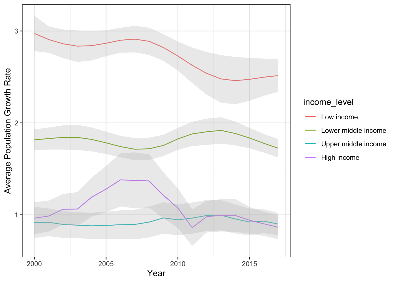
  summarise(mean_se(growth_rate)) #calculates mean + standard error of the mean.

Now, we have the average (+/- standard error) population growth rate for countries at each income level across each year for 2000 to 2017. Here, the mean is “y” and lower and upper standard error is “ymin” and “ymax”, respectively. Let’s plot this. Let’s start with a simple line graph:

ggplot(popgrowth_income, aes(x=as.numeric(year), y=y, group=income_level)) +
  geom_line(aes(color=income_level)) +
  theme_bw()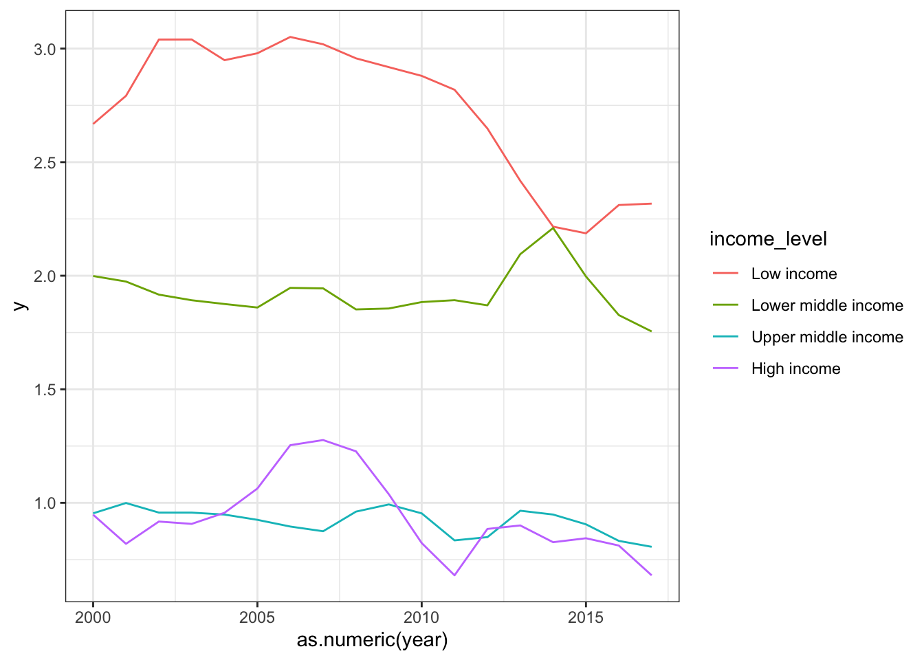

We can make this fancy by adding the confidence band using geom_ribbon(), and cleaning up the axis labels:

ggplot(popgrowth_income, aes(x=as.numeric(year), y=y, group=income_level)) +
  geom_line(aes(color=income_level)) +
  geom_ribbon(aes(ymin=ymin, ymax=ymax), alpha=0.3, fill="gray") +
  theme_bw() +
  ylab("Average Population Growth Rate") +
  xlab("Year")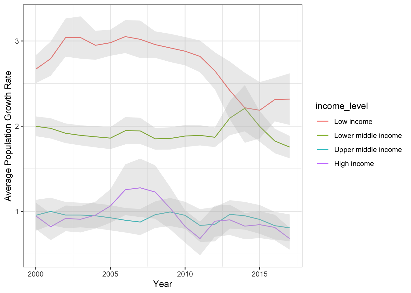

5. How does the relationship between population growth rate and income level differ between global regions?

Now, let’s look at how income levels have different effects on population growth rates depending on the region of the world. to do this, we have to pick a year to analyze. Let’s go with the latest data, 2017.

We can do that simply by going from the original popdat_countries (the raw data with the “aggregates” removed), then filtering it to just the data on population growth, then just looking at the 2017 data for each country. We’ll also keep the region and income level data. We’ll remove rows that have NAs.

popdat_countries %>% 
  dplyr::filter(indicator=="SP.POP.GROW") %>%
  select(country, `2017`, region, income_level) %>%
  drop_na()

## # A tibble: 216 × 4
##    country  `2017` region                     income_level       
##    <chr>     <dbl> <chr>                      <fct>              
##  1 ABW      0.537  Latin America & Caribbean  High income        
##  2 AFG      2.87   South Asia                 Low income         
##  3 AGO      3.55   Sub-Saharan Africa         Lower middle income
##  4 ALB     -0.0920 Europe & Central Asia      Upper middle income
##  5 AND      1.77   Europe & Central Asia      High income        
##  6 ARE      0.820  Middle East & North Africa High income        
##  7 ARG      1.04   Latin America & Caribbean  Upper middle income
##  8 ARM     -0.487  Europe & Central Asia      Upper middle income
##  9 ASM     -1.97   East Asia & Pacific        High income        
## 10 ATG      0.611  Latin America & Caribbean  High income        
## # ℹ 206 more rows

Ok, that looks like what we want, so I’ll save it as popdat_2017:

popdat_2017=popdat_countries %>% 
  dplyr::filter(indicator=="SP.POP.GROW") %>%
  select(country, `2017`, region, income_level) %>%
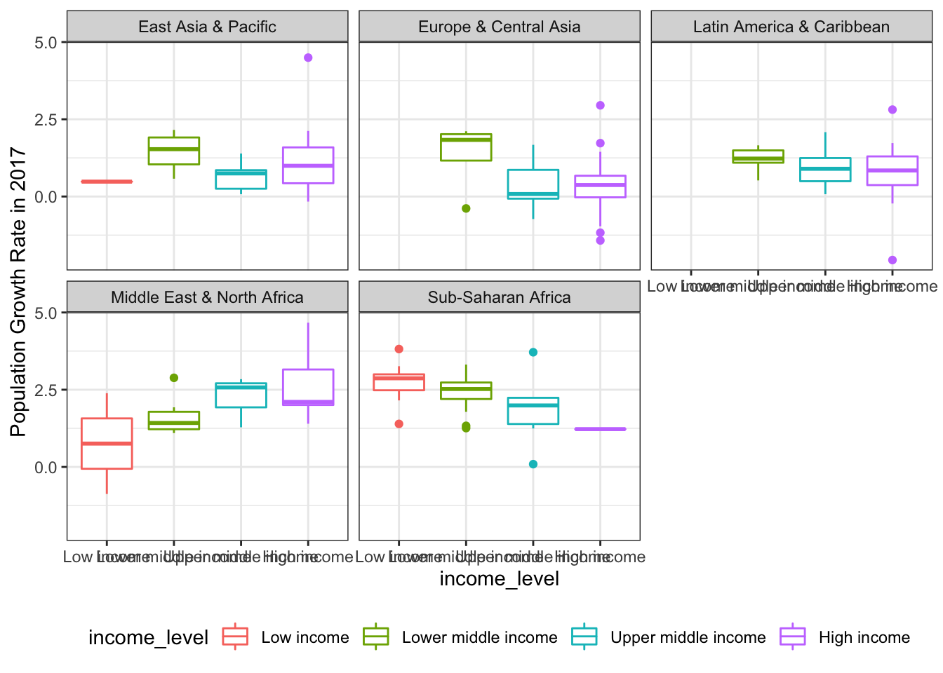
  drop_na()

Now we can plot population growth by income level, and use region to create facets. Here, I’m going to use income_level as both the x axis and color because the x-axis label is going to be hard to read.

ggplot(popdat_2017, aes(x=income_level, y=`2017`)) +
  geom_boxplot(aes(color=income_level)) +
  facet_wrap(~region, nrow=3)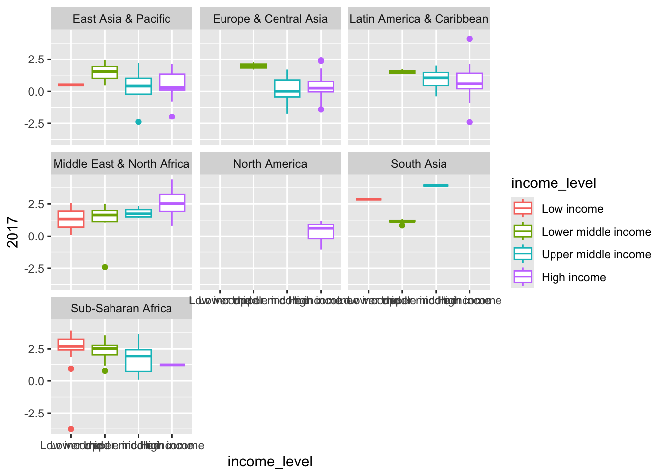

I can see that some regions don’t have enough variation in income level to be useful (e.g., North America and South Asia). I can actually filter the data within the ggplot function to remove those:

Lower income countries have higher population growth rate than those with high income in some regions (sub-Saharan Africa), while in others growth rate is bigger for high earners.

ggplot(popdat_2017 %>% dplyr::filter(region!="North America" & region!="South Asia"), aes(x=income_level, y=`2017`)) +
  geom_boxplot(aes(color=income_level)) +
  facet_wrap(~region, nrow=2) +
  theme_bw() +
  theme(legend.position = "bottom") +
  ylab("Population Growth Rate in 2017")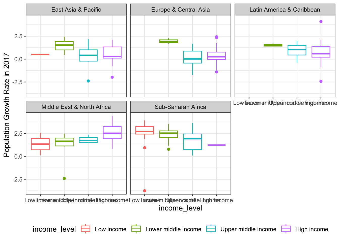

It looks like the relationship between income level and population growth rate indeed changes between regions. For example, in Europe/Central Asia, Latin America/Caribbean, and Sub-Saharan Africa, countries with lower income have higher population growth rate. But the relationship is opposite in the Middle East & North Africa. There, the countries with higher incomes have higher population growth rate.

How would we test the idea that the relationship between income level and population growth rate depends on the region? One way is to run a linear model including the interaction effect of the two variables:

lm.fit=lm(`2017`~region*income_level, data=popdat_2017)

anova(lm.fit)

## Analysis of Variance Table
## 
## Response: 2017
##                      Df  Sum Sq Mean Sq F value    Pr(>F)    
## region                6 119.947 19.9911 18.2739 < 2.2e-16 ***
## income_level          3   5.585  1.8616  1.7017  0.168022    
## region:income_level  12  34.682  2.8902  2.6419  0.002691 ** 
## Residuals           194 212.231  1.0940                      
## ---
## Signif. codes:  0 '***' 0.001 '**' 0.01 '*' 0.05 '.' 0.1 ' ' 1

Worked Example: Wrangling World Bank Population Data

Dai Shizuka

updated 11/05/24

Things you will learn in this Worked Example

Set up: load packages

1. The Data: Population growth trends across the world

`world_bank_pop`: Population data from World Bank (2000-2017)

2. Exclude aggregate data to get data for countries only

3. Which are the world’s largest countries (in 2017)?

4. How population growth rates have changed across years, by income level of countries

5. How does the relationship between population growth rate and income level differ between global regions?

Worked Example: Wrangling World Bank Population Data

Dai Shizuka

updated 11/05/24

Things you will learn in this Worked Example

Set up: load packages

1. The Data: Population growth trends across the world

world_bank_pop: Population data from World Bank (2000-2017)

2. Exclude aggregate data to get data for countries only

3. Which are the world’s largest countries (in 2017)?

4. How population growth rates have changed across years, by income level of countries

5. How does the relationship between population growth rate and income level differ between global regions?

`world_bank_pop`: Population data from World Bank (2000-2017)